The Jackknife and Bootstrap

3 Methods: the jackknife and bootstrap

A statistic $\hat{\theta}$ that we are interested in is a function of the sample $X$:

$$\hat{\theta} = s(X). \tag{12}$$

Bootstrap is designed to get the standard deviation of $\hat{\theta}$ using new samples generated from the original sample $X$. To understand bootstrap, we can start with jackknife first.

3.1 The jackknife estimate of standard error

The basic idea of jackknife is to create new samples from the observed sample using the method of removing one observation at a time.

Define the $i$^th^ jackknife sample as the remaining sample after dropping the $i$th sample, that is

$$X_{(i)} = (X_i, X_2, ..., X_{i-1},X_{i+1}, ...,X_n)', ~~~~~~ \text{for} ~ i = 1, 2, ..., n. \tag{13}$$

The corresponding value of the statistic of interest can be obtained from these jackknife samples as

$$\hat{\theta}_{(i)} = s(X_{(i)}), ~~~~~~ \text{for} ~ i = 1, 2, ..., n. \tag{14}$$

From these $n$ new statistics, the jackknife estimate of standard error for $\hat{\theta}$ can be calculated as

$$\hat{se}_{jack} = \sqrt {\frac{n-1}{n} \sum_1^n \left( \hat{\theta}_{(i)} - \frac{\sum_{i = 1}^n \hat{\theta}_{(i)}}{n} \right)^2}. \tag{15}$$

Take the sample mean $\bar{X}$ as an example. To get the jackknife estimate of standard error for $\bar{X}$, we calculate the sample means of $n$ jackknife samples

$$\bar{X}_{(i)} = \frac{X_1 + X_2 + ... + X_{i-1} + X_{i+1} + ... + X_n}{n-1}, ~~~~~~~~ \text{for} ~ i = 1, 2, ..., n. \tag{16}$$

Then the jackknife estimate of standard error for $\bar{X}$ is

$$\hat{se}_{jack} = \sqrt {\frac{n-1}{n} \sum_{i = 1}^n \left( \bar{X}_{(i)} - \frac{\sum_{i = 1}^n \bar{X}_{(i)}}{n} \right)^2}. \tag{17}$$

Substitute equation $(16)$ into equation $(17)$ and use $\bar{X}$ to denote the original sample mean, we get

$$\hat{se}_{jack} = \sqrt {\frac{\sum_{i = 1}^n(X_i - \bar X)^2}{n(n-1)}}, \tag{18}$$

which is exactly the same form as the classic formula.

3.2 The nonparametric bootstrap estimate of standard error

The jackknife approach does not work for unsmooth statistics while bootstrap does not have these drawbacks. More details about the features of jackknife and bootstrap can be found in Efron and Hastie’s (2016) book. The difference between bootstrap samples from jackknife samples is that bootstrap samples are obtained from random sampling with replacement. Apart from this, instead of $n$ new samples, there can be any number of bootstrap samples. Though 200 bootstrap samples would be sufficient for the estimate of standard error (Efron and Tibshirani, 1993). The sample size of a bootstrap sample is $n$, the same as the original sample.

Let the number of bootstrap samples be $B$. Then denote the $i$^th^ bootstrap sample as

$$X^*_{(i)} = (X^*_1, X^*_2, ..., X^*_n), ~~~~~~ \text{for} ~ i = 1, 2, ..., B. \tag{19}$$

Similarly, the corresponding value of the statistic of interest can be obtained as

$$\hat{\theta}^*_{(i)} = s(X_{(i)}^*), ~~~~~~ \text{for} ~ i = 1, 2, ..., B. \tag{20}$$

The bootstrap estimate of standard error for $\hat{\theta}$ is then the empirical standard deviation of these $B$ values,

$$\hat{se}_{boot} = \sqrt{\frac{\sum_1^B \left( \hat{\theta}^*_{(i)} - \frac{\sum_1^N \hat{\theta}^*_{(i)}}{B} \right)^2}{B-1}}. \tag{21}$$

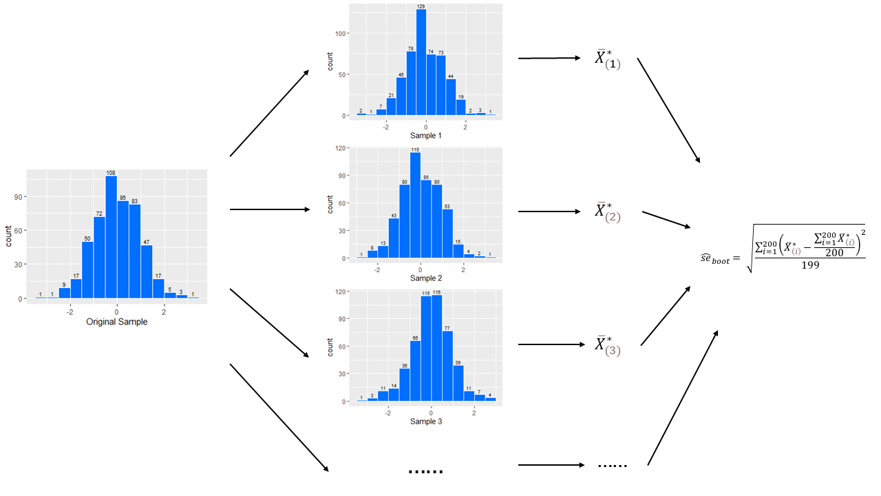
Take a dataset of 500 uncorrelated data from the standard normal distribution as an example.

As shown in Figure 2,

• Randomly obtain 500 data with replacement from the dataset as Sample 1.

• Then repeat this procedure $B$ times ($B = 200$ is used in this example) to get Sample 2, Sample 3, …

• Calculate the corresponding statistics of interest of these samples. The sample mean is used in this example.

• Bootstrap estimate of standard error for this statistic then can be calculated.

Figure 2: The process of Bootstrap applied for example data set

3.3 Resampling Plans

The jackknife and the bootstrap are both specific situations of resampling from the original sample $X = (X_1, X_2, ..., X_n)'$.

3.3.1 Resampling Vector

Define a resampling vector $\mathbf{P} = (P_1, P_2, ..., P_n)$, in which $P_i \geq 0$ and $\sum_{i=1}^{n} P_i = 1$.

$P_i$ in the vector $\mathbf{P}$ means how much $X_i$ weights in the new sample:

$$P_i = \frac{\text{The number of} ~ X_i ~ \text{in the new sample}}{\text{The sample size of the new sample}}. \tag{22}$$

Therefore, the information in the new sample can be obtained entirely from $P$ and the original sample vector $X = (X_1, X_2, ..., X_n)'$.

The set of all possible values of $P_i$ is a space which is a simplex ¹ denoted by $S_n$.

The new sample can be totally obtained from resampling vector $\mathbf{P}$ with the original sample $X$ fixed. Thus, the statistic of interest $\hat{\theta}^*$ corresponding to this specific new sample can be written as a function of $\mathbf{P}$:

$$\hat{\theta}^* = S(\mathbf{P}). \tag{23}$$

The resampling plans intends to find out how the statistic of interest $\hat{\theta}^*$ changes with the weight vector $\mathbf{P}$ varies across its value space, namely $S_n$, holding the original data set $X$ fixed.

3.3.2 Resampling vectors of jackknife samples and bootstrap samples

Let the resampling vector with equal weight on each $X_i$ be

$$\mathbf{P}_0 = \frac{(\overbrace{1, 1, ..., 1}^{n ~ in ~ total})'}{n}. \tag{24}$$

The sample corresponding to $\mathbf{P}_0$ is exactly the same as the original sample $X$. Then we have

$$S(\mathbf{P}_0) = s(X) = \hat{\theta}, \tag{25}$$

which is the original estimate of the statistic of interest.

The resampling vector of the $i$^th^ jackknife sample $X_{(i)}$ is

$$\mathbf{P}_{(i)} = \frac{(\overbrace{1, 1, ..., 1}^{i-1}, 0, \overbrace{1, 1, ..., 1}^{n-i})'}{n-1}. \tag{26}$$

For the $i$^th^ bootstrap sample $X^*_{(i)}$, the resampling vector is

$$\mathbf{P}^*_{(i)} = \frac{(N_1, N_2, ..., N_n)'}{n}, \tag{27}$$

where $N_i$ denotes the number of $X_i$ (the $i$^th^ observation from the original sample) in the new sample. Therefore we will have $\sum_1^n N_i = n$.

What we do to get a bootstrap sample is to draw $n$ times from $n$ observations, and the probability of each observation being drawn is 1/n. Thus the outcome $(N_1, N_2, ..., N_n)'$ follows a multinomial distribution. Therefore, for each specific value of $\mathbf{P}^*_{(i)}$, the probability of getting its corresponding sample denoted bootstrap probability can be calculated.

3.3.3 An Example of Resampling Simplex for Sample of Size 3

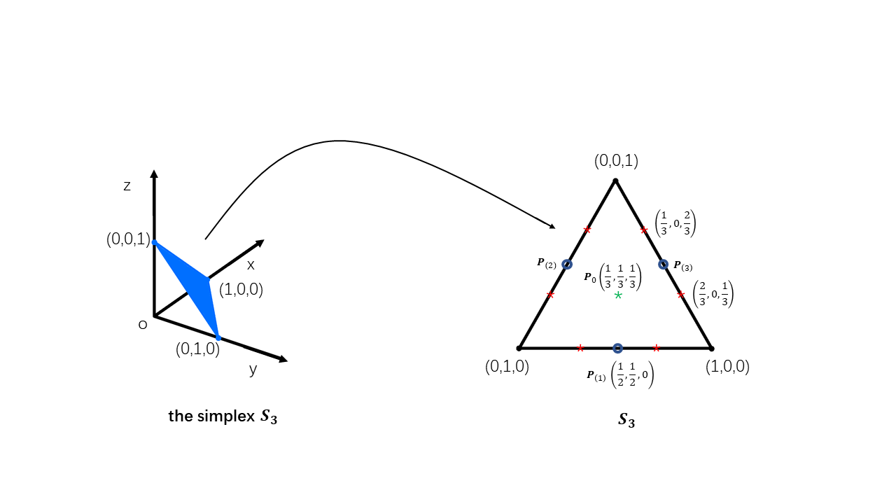
Figure 3 demonstrates a resampling simplex for the original sample with $3$ observations $X = (X_1, X_2, X_3)'$.

The centre point is $\mathbf{P}_0$ with the same weight for these $3$ observations. $\mathbf{P}_{(1)}$, $\mathbf{P}_{(2)}$ and $\mathbf{P}_{(3)}$ are the jackknife points. For each jackknife point, the one observation removed has weight 0 while the remaining two both weigh $1/2$.

As for bootstrap, there are 10 possible situations for its new samples which are $\mathbf{P}_0$, the three corner points and the six red starred points. The probability of obtaining these samples is different. Ideally, in every $27$ samples, there will be $6$ centre points ($\mathbf{P}_0$), $1$ for each of the $3$ corner points and $3$ for each of the $6$ red starred points.

Figure 3: An example of a resampling simplex for sample size n = 3

3.3.4 The statistic of interest corresponding to the resampling vector

To explore the relationship between the statistic of interest $\hat{\theta}^*$ and the resampling vector $\mathbf{P}$ is to study the features of the function between them which is $\hat{\theta}^* = S(\mathbf{P})$.

The Euclidean distance between a jackknife vector $\mathbf{P}_{(i)}$ and $\mathbf{P}_0$ is

$$\| \mathbf{P}_{(i)} - \mathbf{P}_{0} \| = \frac{1}{\sqrt{n(n-1)}}. \tag{28}$$

With bootstrap probability known, the expected root mean square distance between a bootstrap vector $\mathbf{P}^*_{(i)}$ and $\mathbf{P}_0$ can be calculated as well:

$${\left( E {\| \mathbf{P}^*_{(i)} - \mathbf{P}_{0}} \|^2 \right)}^{\frac{1}{2}} = \sqrt{\frac{n-1}{n^2}}. \tag{29}$$

From above we can get that the expected distance between a bootstrap vector and the centre is an order of magnitude $\sqrt{n}$ times further than the centre distance of a jackknife vector.

The approximate directional derivative of $S(\mathbf{P})$ in the direction from $\mathbf{P}_{(i)}$ to $\mathbf{P}_0$ is

$$D_i = \frac{ S(\mathbf{P}_{(i)}) - S({\mathbf{P}_{0})} }{\| \mathbf{P}_{(i)} - \mathbf{P}_{0} \|} = \left( \hat{\theta}_{(i)} - \frac{\sum_1^n \hat{\theta}_{(i)}}{n} \right) \left( \sqrt{n(n-1)} \right), \tag{30}$$

which means the slope of function $S(\mathbf{P})$ at $\mathbf{P}_0$ in the direction of $\mathbf{P}_{(i)}$.

Compare it with the formula of the jackknife estimate of standard error for $\hat{\theta}$ ($\hat{se}_{jack}$), we can find that $\hat{se}_{jack}$ is proportional to the root mean square of the slopes $D_i$.

When $S(\mathbf{P})$ is a linear function of $\mathbf{P}$, like the sample mean, $\hat{se}_{jack}$ is equal to $\hat{se}_{boot}$. And when $S(\mathbf{P})$ is not linear, $\hat{se}_{jack}$ is only an approximation (Efron and Hastie, 2016).

3.3.5 Compromise of the bootstrap algorithm

Theoretically, for a specific original sample set, with the distribution of all the possible bootstrap vectors known, the ideal bootstrap standard error estimate can be evaluated.

For a sample set with $K$ possible resampling points, the ideal bootstrap standard error estimate is

$$\hat{se}_{boot} = \sqrt{ \sum_{i = 1}^K p_k \left( S(\mathbf{P}_{(k)}^*) - S(\mathbf{P}_{0}) \right)^2 }, \tag{31}$$

where $p_k$ is the bootstrap probability corresponding to $\mathbf{P}_{(k)}^*$. In this situation, the weighted mean of these $K$ resampling points is the same as $S(\mathbf{P}_{0})$.

However, the number of the possible resampling points $K$ increase incredibly with the increase of the sample size $n$. For a sample of size n

$$K = \begin{pmatrix} 2n-1 \\\\ n \end{pmatrix}. \tag{32}$$

For $n = 20$, the number of $K$ comes to $6.9 \times 10^{10}$ already. Thus it is unrealistic to calculate the ideal bootstrap standard error estimate in real life. What we do is to choose $B$ resampling vectors at random, as mentioned in the former part, to get a sufficiently accurate estimate.

References

Efron, B., Hastie, T. (2016) The Jackknife and the Bootstrap, Computer age statistical inference Algorithms, evidence, and data science. Cambridge: Cambridge University Press, pp. 155-166.

Footnotes

1. A $(n - 1)$-dimensional simplex ($S_n$) is a set of nonnegative vectors summing to 1. More details of simplex can be found in Weisstein, E. W. “Simplex.” Accessed March 22^th^ 2021. MathWorld—A Wolfram Web Resource. https://mathworld.wolfram.com/Simplex.html. ↩