Functional Data Analysis Notes 3 - Functional PCA

阅读材料：Ramsay, J.O., Silverman, B.W. (2005) Functional Data Analysis (2nd Edition) Section 8.1-8.6, 9.1-9.4.

1 Multivariate Principal Components Analysis

The basic idea of Principal Components Analysis is to transform a group of potentially correlated variables into a group of linearly uncorrelated variables through orthogonal transformation, and this group of variables after conversion are called principal components.

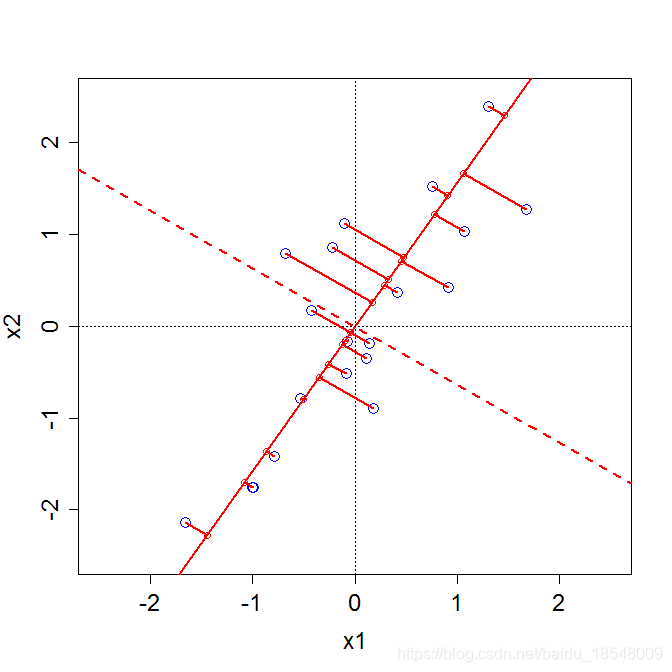
1.1 A little analysis

• Measure total variation in the data as total squared distance from center: $\sum_{j=1}^d \sum_{i=1}^{n} (x_{ij} - \bar{x}_j)^2 = trace[\Sigma];$
• If $x$ has covariance $\Sigma$, the variance of $u^Tx$ is $u^T \Sigma u$;
• To maximize $u^T \Sigma u$ (or $u^Tu$) we solve the eigen-equation $\Sigma u = \lambda u;$
• For $u^Tu = 1$, the closest multiple of $u$ to $x-\bar{x}$ is $(u^Tu)^{-1} (u^Tx)u = (u^T(x-\bar{x}))u.$

1.2 Mechanics of PCA

For an $n \times p$ data matrix with $n$ observations and $p$ attributions:

• Estimate the covariance matrix (using sample covariance matrix) $\Sigma = \frac{1}{n-1} (X - \bar{X})^T(X - \bar{X}),$ where $\bar{X}$ is the mean vector of the $p$ attributions of the data matrix $X$;
• Take the eigen-decomposition of $\Sigma$ $\Sigma = U^TDU = \sum d_{ii} u_i u_i^T;$
  • Columns of $U$ are orthogonal; represent a new basis. Denoting the $i$^th^ column of $U$ by $u_i$;
  • $D$ is a diagonal matrix. Its entries ($d_{ii}$) (eigenvalues) give variances of data along corresponding directions $U$.
• Order $D$, $U$ in terms of decreasing $d_{ii}$;
• $(X - \bar{X})^T u_i$ is the $i$^th^ principal component score.

2 Functional PCA

2.1 Re-interpretation

Instead of covariance matrix $\Sigma$, we have a surface $\sigma (s, t)$.

Re-interpret eigen-decomposition:

$\Sigma = U^TDU = \sum d_{ii} u_i u_i^T.$

For functions, this is the Karhunen-Loève decomposition:

$\sigma (s, t) = \sum_{i=1}^{\infty} d_{ii} \xi_i (s) \xi_i (t),$

where

• $d_{ii}$ represents amount of variation in direction $\xi_i (t)$;
• $\int \xi_i (t)^2 dt = I.$ (??)

For the collection of curves $x_i (t)$, $i = 1, ..., n$, we want to find the probe $\xi_1 (t)$ that maximizes

$Var \bigg[ \int \xi_1 (t) x_i (t) dt \bigg].$

But we need to constrain $\int \xi_1 (t)^2 dt = 1$.

For $\xi_2 (t)$ we want to maximize the variance subject to the orthogonality condition $\int \xi_1 (t) \xi_2(t) dt = 0$

For $\xi_1, ..., \xi_d$ best approximation to $x(t)$ is

\hat{x} (t) &= \bar{x} (t) + \bigg( \int \Big( x(t) - \bar{x} (t) \Big) \xi_1 (t) ~ dt \bigg) \xi_1 (t) + ... \\\\ &~~~~~ + \bigg( \int \Big( x(t) - \bar{x} (t) \Big) \xi_d (t) ~ dt \bigg) \xi_d (t) \\\\ &= f_1 \xi_1 (t) + ... + f_d \xi_d (t). \end{aligned}$$ which can be seen as a new basis! For $\hat{y} = g_1 \xi_1 (t) + ... + g_d \xi_d(t)$: $$\int \big( \hat{x}(t) - \hat{y} (t) \big)^2 ~ dt = \sum_{i=1}^d (f_i - g_i)^2.$$ The covariance surface can be decomposed: $$\sigma (s, t) = \sum_{i=1}^\infty d_{ii} \xi_i (s) \xi_i (t)$$ with the $\xi_i$ orthonormal. * The $\xi_i (t)$ are the principal components; successively maximize $Var_i \big[ \int \xi_i (t) x_j (t) ~ dt \big]$. * $d_{ii} = Var_i \big[ \int \xi_i (t) x_j (t) ~ dt \big]$. * $d_{ii} / \sum d_{ii}$ is proportion of variance explained. * $\xi_1, ...$ is a basis system specifically designed for the $x_i (t)$. * Principal component scores are $$f_{ij} = \int \xi_i (t) [x_j(t) - \bar{x}(t)] ~ dt$$ * Reconstrction of $x_i (t)$: $$x_i (t) = \bar{x} (t) + \sum_{j = 1}^{\infty} f_{ij} \xi_j (t)$$ ### 2.2 Computing FPCA Components solve the eigen-equation: $$\int \sigma (s, t) \xi_i (t) ~ dt = \lambda \xi_i (t)$$ Option 1: 1. take a fine grid $\mathbf{t} = [t_1, ..., t_K]$ 2. find the eigen-decomposition of $\Sigma (\mathbf{t}, \mathbf{t})$ 3. interpolate the eigenvectors Option 2 (in *fda* library): 1. if the $x_i(t)$ have a common basis expansion, so must the eigen-functions; 2. can re-express eigen-equation in terms of co-efficients; 3. basis expansion will become apparent for smaller eigenvalues.      ### 2.3 Varimax rotations A set of principal components defines a **subspace**. Within that space, we can try to find a more interpretable basis. That amounts to a rotation of the coordinate axes. The basic idea is to try to find coordinate system where PC loadings are either very large or very small. The varimax criterion is $$maximize \sum Var(u_i^2).$$ ### 2.4 Summary * PCA = means of summarizing high dimensional covariation; * fPCA = extension to infinite-dimensional covariation; * Representation terms of basis functions for fast(er) computation; * Varimax rotations = focus on particular regions; nice display properties. ## 3 Smoothed PCA ### 3.1 A general perspective of PCA For observations $x_1, x_2, ..., x_n$ (vectors, functions, ...), we want to find $\xi_1$ so that $$\sum \| x_i - <x_i, \xi_1> \xi_1 \|$$ is as small as possible. $<x_i, \xi_1>$ is the best multiplier of $\xi_1$ to fit $x_i$. Now we want $\xi_2$ to be the next best such that $<\xi_2, \xi_1> = 0$. #### 3.1.1 Inner product Vectors are otrhogonal if they intersect at right angles. $\mathbf{x}$ and $\mathbf{y}$ are orthogonal if $\mathbf{x}^T \mathbf{y} = 0$ (i.e. $\sum x_i y_i = 0$). In order to deal with $x(t)$ that are functions, multivariate functions, or mixed functions and scalars, we need a more general notation. This will also help us understand smoothing a little more. An inner produnct is a symmetric bilinear operator <., .> on a vector space $\mathcal{F}$ taking values in $\mathbb{R}$: * $<x, y> = <y, x>$; *(symmetry)* * $<ax, y> = a <x, y>$; * $<x+y, z> = <x, z> + <y, z>$; *(linearity for one element)* * $<x, x> ~ > 0$ with $x$ a non-zero vector. *(positivity)* For example: * Euclidean space: $<x, y> = x^Ty$. * $\mathcal{L}^2 (\mathbb{R})$: $\int x(t) y(t) ~ dt$. Associated notion of distance or size: $$\| x - y \| = < x - y, x - y>.$$ So to get to $x$ as close as possible in the direction $y$: $$\min_a <x - ay, x - ay>,$$ which is solved at $$a = <x, y> / <y, y>.$$ If $<y, y> = 1$, $<x, y>$ is a measure of commonality. If $<y, z> = 0$ minimum of $\| x - ay - bz \|$ at $$a = <x, y>, ~ b = <x, z>.$$ #### 3.1.2 Inner produncts and PCA For a collection $x_1, x_2, ..., x_n$, seek a probe $\xi$ to maximize $$Var[<\xi, x_i>].$$ Require $<\xi_i, \xi_j> = \delta_{ij}$. Implies optimal reconstruction:

\left[ \begin{matrix} <x_1, \xi_1> & \cdots & <x_1, \xi_d> \ \vdots & & \vdots\ <x_n, \xi_1> & \cdots & <x_n, \xi_d> \end{matrix} \right],

best summarization of $x_1, ..., x_n$ with $d$ numbers. #### 3.1.3 Defining new inner products For a multivariate function $\mathbf{x}(t) = \big( x_1(t), x_2(t) \big)$. A new inner product is $$<(x_1, x_2), (y_1, y_2)> = <x_1, y_1> + <x_2, y_2>,$$ which can be check that this is a bilinear form. Note that $$<\big( x_1 (t), x_2 (t) \big), \big( y_1 (t), y_2 (t) \big) > = 0$$ does **NOT** imply $$<x_1, y_1> = 0 ~~ and ~~ <x_2, y_2> = 0$$ #### 3.1.4 fPCA with multivariate functions If we have $x_i(t)$ and $y_i(t)$, $i = 1, ..., n$. Then we want to find $\big( \xi_x (t), \xi_y (t) \big)$ to maximize $$Var \bigg[ \int \xi_x (t) x_i (t) ~ dt + \int \xi_y (t) y_i (t) ~ dt \bigg].$$ This is like putting $x$ and $y$ together end-to-end:

z(t) = \begin{cases} x(t), ~~~ t \leq T \ y(t), ~~~ t > T \end{cases}~~.

### 3.2 Smoothing and fPCA When observed functions are rough, we may want the PCA to be smooth * reduces high-frequency variation in the $x_i(t)$; * provides better reconstruction of future $x_i(t)$. We therefore want to find a way to impose smoothness on the principal components. #### 3.2.1 Including derivatives Consider the multivariate function $\big( x(t), Lx(t) \big)$, where $Lx(t)$ is the acceleration function (i.e. a function of $D^n x(t)$ ). Inner product: $$\begin{aligned} <x, y> &= < \big( x(t), Lx(t)), (y(t), Ly(t) \big) > \\\\ &= \int x(t) y(t) ~ dt + \lambda \int Lx(t) Ly(t)n ~ dt. \end{aligned}$$ Smoothing: * think of $\mathbf{y} = \big( y_1 (t), y_2 (t) \big) = \big( y(t), 0 \big)$; * try to fit with $\mathbf{x} = \big( x(t), Lx(t) \big)$; * but the norm is defined by the Sobolev inner product above. #### 3.2.2 A new measure of size Usually, we measure size in the $L^2$ norm $$\| \xi (t) \|_2^2 = \int \xi (t)^2 ~ dt.$$ But penalization methods implicitly use a ***Sobolev norm**: $$\| \xi(t) \|_L^2 = \int \xi (t)^2 ~ dt + \lambda \int [L \xi(t)]^2 ~ dt.$$ Search for the $\xi$ that maximizes $$\frac{Var \big[ \int \xi(t) x_i (t) ~ dt \big]}{\| \xi(t) \|_L^2} = \frac{Var \big[ \int \xi(t) x_i (t) ~ dt \big]}{\int \xi (t)^2 dt + \lambda \int \big[ L \xi (t) \big]^2dt}.$$ #### 3.2.3 Size and orthogonality * As $\lambda$ increases, emphasize making $L \xi(t)$ small over maximizing the variance. * Successive $\xi_i$ now satisfy $$\int \xi_i (t) \xi_j dt + \lambda \int L \xi_i (t) L \xi_j (t) dt = 0.$$ * Effectively "pretending" that $Lx_i(t) = 0$. * Coeffiicients of best (in least-squares sense) fit no longer $\int \xi_i (t) x_j (t) dt$. * Best fit coefficents now also depend on which eigenfunctions are used. ### 3.3 Summary * Multivariate and Mixed PCs – like extending the vector; * Need to think about weighting; * Smoothing: may be done through a new inner product; * Cross Validation: objective way to work out if smoothing is doing anything useful for you; * Can use fPCA to help reconstruct partially-observed functions ## 4 Research papers Liu, C., Ray, S., Hooker, G. and Friedl, M. (201), Functional principal component and factor analysis of spatially correlated data, *Statistics and Computing* Liu, C., Ray, S., Hooker, G. and Friedl, M. (2012), Functional factor analysis for periodic remote sensing data, *The Annals of Applied Statistics* 6(2), 601–624. Paul, D. and Peng, J. (2011), Principal components analysis for sparsely observed correlated functional data using kernel smoothing method. *Electronic Journal of Statistics* (5). Yao, F., Muller, H. and Wang, J. (2005), Functional data analysis for sparse longitudinal data, *Journal of the American Statistical Association* 100(470), 577–590.