Functional Data Analysis Notes 2 - Smoothing and Descriptive Statistics

阅读材料：Ramsay, J.O., Silverman, B.W. (2005) Functional Data Analysis (2nd Edition) Section 4.1, 4.2, 4.3, 4.4, 4.5, 5.1, 5.2, 5.3, 5.4 and 5.5.

1 Fitting and smoothing

1.1 Fitted by least squares

For a single curve

$y_i = x(t_i) + \epsilon,$

we want to estimate

$x(t) \approx \sum_{j=1}^k c_j \phi_j (t).$

Minimize the sum of squared errors:

$SSE = \sum_{i=1}^n (y_i - x(t_i))^2 = \sum_{i=1}^n (y_i - \mathbf{c}^T \Phi (t_i))^2,$

where

$\mathbf{c}_{k \times1} = (c_1, c_2, ..., c_j, ..., c_k)^T,$

$\Phi_{k \times 1}(t_i) = \big( \phi_1(t_i), \phi_2(t_i), ..., \phi_j(t_i), ..., \phi_k(t_i) \big)^T.$

Denote

$\mathbf{y}_{n \times 1} = (y_1, y_2, ..., y_i, ..., y_n)^T,$

$$\begin{aligned} \mathbf{\Phi}_{n \times k} &= ~~ \left( \begin{array}{ccc} ~ \Phi(t_1), & ~ \Phi(t_2), & \ldots, ~ & \Phi(t_i), & \ldots, ~ & \Phi(t_n) ~ \\ \end{array} \right) \\ {} \\ &= \left( \begin{array}{ccc} \phi_1(t_1), & \phi_1(t_2), & \ldots, & \phi_1(t_i), & \ldots, & \phi_1(t_n) \\ \phi_2(t_1), & \phi_2(t_2), & \ldots, & \phi_2(t_i), & \ldots, & \phi_2(t_n) \\ \vdots & \vdots & & \vdots & & \vdots\\ \phi_j(t_1), & \phi_j(t_2), & \ldots, & \phi_j(t_i), & \ldots, & \phi_j(t_n) \\ \vdots & \vdots & & \vdots & & \vdots\\ \phi_k(t_1), & \phi_k(t_2), & \ldots, & \phi_k(t_i), & \ldots, & \phi_k(t_n) \\ \end{array} \right) \end{aligned}.$$

Then we can write

$SSE(\mathbf{c}) = (\mathbf{y} - \mathbf{\Phi c})^T (\mathbf{y} - \mathbf{\Phi c}).$

The ordinary least squares estimate is

$$\begin{aligned} \hat{\mathbf{c}} &= argmin (\mathbf{y} - \mathbf{\Phi c})^T (\mathbf{y} - \mathbf{\Phi c}) \\ &= (\mathbf{\Phi}^T \mathbf{\Phi})^{-1} \mathbf{\Phi}^T \mathbf{y} \end{aligned}.$$

Then we have the estimate

$\hat{x}(t) = \Phi_{1 \times k} (t) \cdot \hat{\mathbf{c}} = \Phi (t) \cdot \overbrace{(\mathbf{\Phi}^T \mathbf{\Phi})^{-1} \mathbf{\Phi}^T \mathbf{y}}^{k \times 1}.$

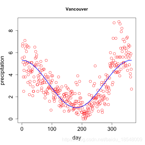
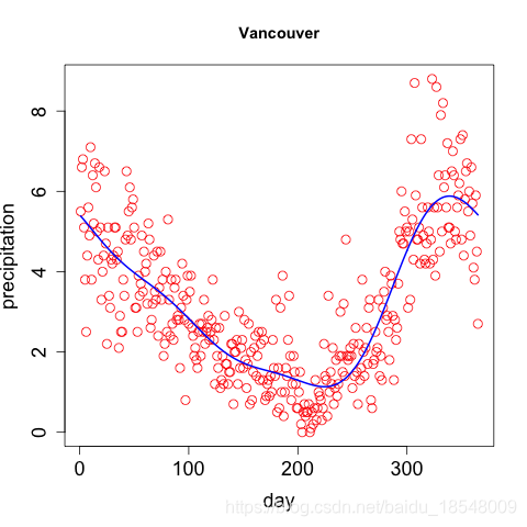
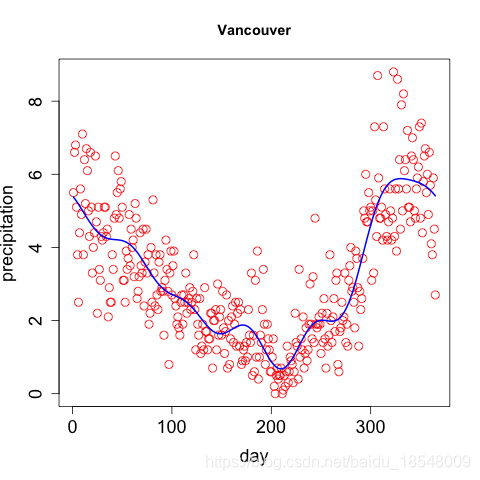
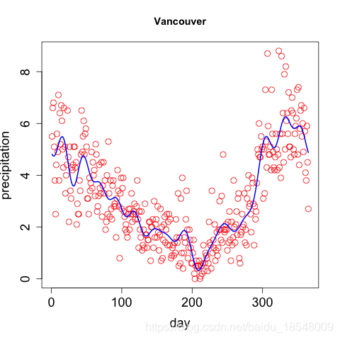
1.2 Choosing the number of basis functions

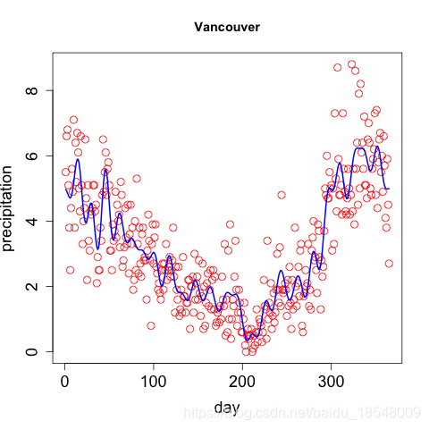
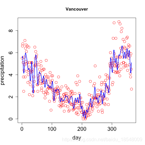
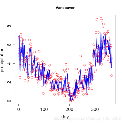
• Trade off:

  fails to capture interesting features of the curves	$\stackrel{\mathrm{the ~ number ~ of ~ basis ~ functions ~ (i.e. ~ k)}}{\longleftrightarrow}$	more flexible but “overfit”, reflect errors of measurement

• Spline basis: number of knots $\nearrow$ , the order of the basis $\nearrow$ $\Longrightarrow$ more flexible

Vancouver Precipitation: 3, 7, 13, 31, 53, 105, 209, 365 Fourier Bases

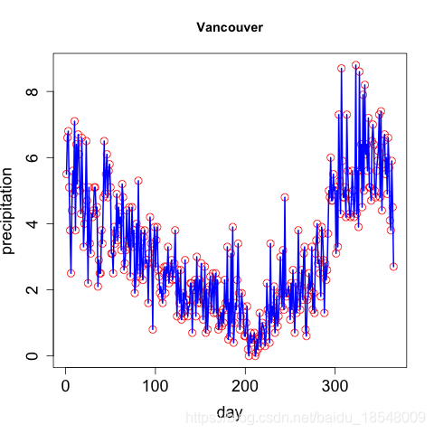This trade-off can be express in terms of

• the bias of the estimate of $x(t)$: $Bias[\hat{x}(t)] = x(t) - E[\hat{x}(t)],$
• the sampling variance of the estimate: $Var[\hat{x}(t)] = E \big[ \{ x(t) - E[\hat{x}(t)] \}^2 \big].$

small bias but large sampling variance	$\stackrel{\mathrm{the ~ number ~ of ~ basis ~ functions ~ (i.e. ~ k)}}{\longleftrightarrow}$	small sampling variance but large bias

Usually, we would really like to minimize mean squared error

$MSE[\hat{x} (x)] = E\big[ \{ \hat{x}(t) - x(t) \}^2 \big].$

There is a simple relationship between MSE and bias/variance

$MSE[\hat{x} (t)] = Bias^2[\hat{x}(t)] + Var[\hat{x}(t)],$ for each value of $t$.

In general, we would like to minimize the integrated mean squared error:

$IMSE[\hat{x} (t)] = \int MSE[\hat{x} (t)] ~ dt.$

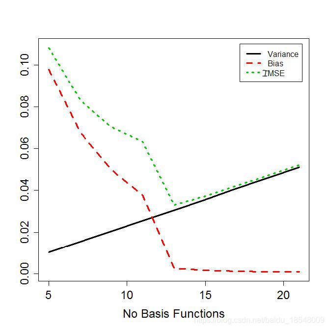
Eg. Bias and variance against $k$ from simulation.

1.3 Cross-validation

One method of choosing a model is through cross validation.

1. leave out one observation $(t_i, y_i)$;

2. estimate $\hat{x}_{-i}(t)$ from remaining data;

3. measure the model’s performance in predicting $t_i$. i.e. $y_i - \hat{x}_{-i}(t_i)$;

4. choose $k$ to minimize the ordinary cross-validation score:

   $OCV[\hat{x}] = \sum \big(y_i - \hat{x}_{-i}(t_i) \big)^2,$

   for a linear smooth $\hat{y} = Sy$

   $OCV[\hat{x}] = \sum \frac{\big(y_i - \hat{x}_{i}(t_i) \big)^2}{(1 - s_{ii})^2}.$

1.4 Summary

• Fitting smooth curves is just linear regression using basis functions as independent variables.
• Trade-off between bias and variance in choosing the number of basis functions $k$.
• Cross-validation is one way to quantitatively find the best number of basis functions.
• Confidence intervals can be calculated using the standard model, but these should be treated with care.

2 Roughness penalty

Some disadvantages of basis expansions:

• Discrete choice of number of basis functions $\Rightarrow$ additional variability;
• Non-hierarchical bases (eg. B-splines) make life more complicated;
• Not necessarily easy to tailor to problems at hand.

2.1 Smoothing penalties

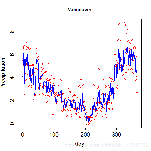
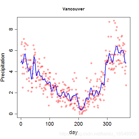
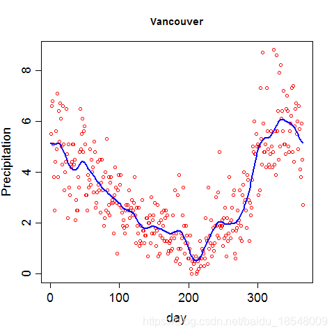
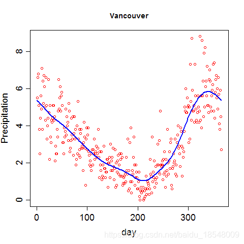
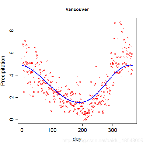
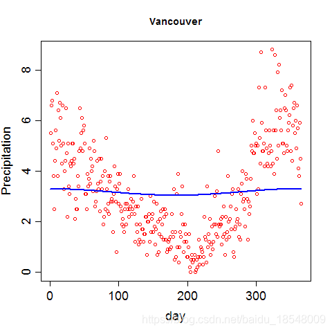
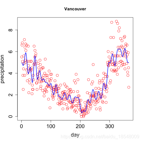
Add a penalty to the least-squares criterion:

$$\begin{aligned} PENSSE_\lambda (x) &= SSE + \lambda J[x] \\ &= [\mathbf{y} - x(\mathbf{t})][\mathbf{y} - x(\mathbf{t})]^T + \lambda J[x], \\ \end{aligned}$$

where

• $J[x]$ measures “roughness” of $x$;
• $\lambda$ is a smoothing parameter measuring compromise between fit and smoothness.
  • $\lambda \rightarrow \infty \Rightarrow$ roughness increase penalty, $x(t)$ becomes smooth.
  • $\lambda \rightarrow 0 \Rightarrow$ penalty reduces, $x(t)$ fits data better.

Experiments with the vancouver weather
log λ = -1	log λ = 3	log λ = 7
log λ = 11	log λ = 15	log λ = 19

## 2.2 The $D$ operator

To increase smoothness is to eliminate small “wiggles” in the data.

For a function $x(t)$, denote

$Dx(t) = \frac{d}{dt} x(t).$ Further derivatives in terms of powers of $D$ is denoted by

$$\begin{aligned} D^2x(t) &= \frac{d^2}{dt^2} x(t), \\\\ &..., \\\\ D^kx(t) &= \frac{d^k}{dt^k} x(t), \\\\ &... \end{aligned}$$

• $Dx(t)$ is the instantaneous slope of $x(t)$; $D^2x(t)$ is its curvature.

• We measure the size of the curvature for all of $f$ by

$J_2(x) = \int \big[ D^2x(t) \big]^2 dt.$

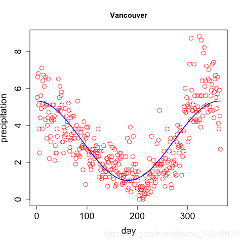
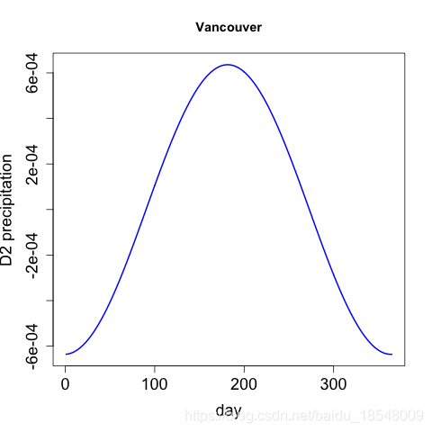
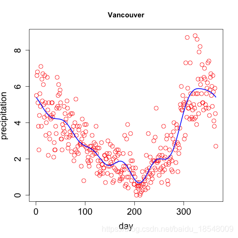
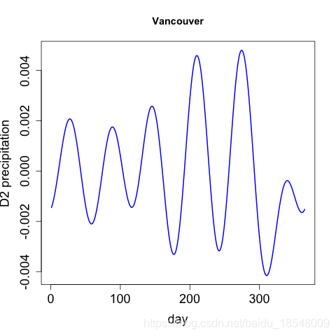
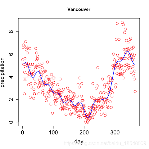
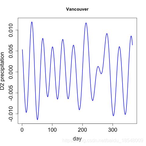
Eg. Curvature of vancouver precipitation

3 Fourier bases:
13 Fourier bases:
25 Fourier bases:

2.3 The roughness of derivatives

Sometimes we may want to examine a derivative of $x(t)$, say $D^2x(t)$.

We then should consider the roughness of that derivative

$D^2 \big[ D^2 x(t) \big] = D^4 x(t).$

This means we measure

$J_4[x] = \int \big[ D^4 x(t) \big]^2 dt.$

And the roughness of the m^th^ derivative is

$J_{m+2}[x] = \int \big[ D^{m+2} x(t) \big]^2 dt.$

2.4 The smoothing spline theorem

Consider the “usual” penalized squared error:

$PENSSE_\lambda (x) = [\mathbf{y} - x(\mathbf{t})]^T [\mathbf{y} - x(\mathbf{t})] + \lambda \int [D^2 x(t)]^2 dt.$

A remarkable theorem tells us that the function $x(t)$ that minimizes $PENSSE_\lambda(x)$ is

• a spline function of order 4 (piecewise cubic),
• with a knot at each sample point $t_j$.

This is often referred to simply as cubic spline smoothing.

As $x(t)$ is of the form

$x(t) = \Phi (t)^T \mathbf{c},$

where $\Phi(t)$ is a $1 \times k$ vector of B-spline basis functions.

The number of basis function (i.e. $k$) is the sum of order ($m$) and the number of interior knots:

$k = 4 + (n - 2) = n + 2.$

Then we need to calculate $c$.

2.4.1 Calculating the penalized fit

When $x(t) = \Phi (t)^T \mathbf{c}$, we have that

$$\begin{aligned} \int \big[ D^m x(t) \big]^2 ~ dt &= \int D^m \big[ \Phi (t)^T \mathbf{c} \big]^T \big[ \Phi (t)^T \mathbf{c} \big] ~ dt \\\\ &= \int \mathbf{c}^T D^m \Phi (t) D^m \Phi (t)^T \mathbf{c} ~ dt \\\\ &= \mathbf{c}^T R \mathbf{c}. \end{aligned}$$

$R$ is known as the penalty matrix.

The penalized least squares estimate for $\mathbf{c}$ is now

$\hat{\mathbf{c}} = \big[ \mathbf{\Phi}^T W \mathbf{\Phi} + \lambda R \big]^{-1} \mathbf{\Phi}^T W \mathbf{y}.$

So we have

$\hat{\mathbf{y}} = \mathbf{\Phi} \hat{\mathbf{c}} = \mathbf{\Phi} \big[ \mathbf{\Phi}^T W \mathbf{\Phi} + \lambda R \big]^{-1} \mathbf{\Phi}^T W \mathbf{y},$

which is still a linear smoother.

2.4.2 More general smoothing penalties

$D^2 x(t)$ is only one way to measure the roughness of $x$.

If we were interested in $D^2 x(t)$, we might think of penalizing $D^4 x(t)$ $\Rightarrow$ cubic polynomials are not rough.

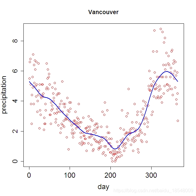
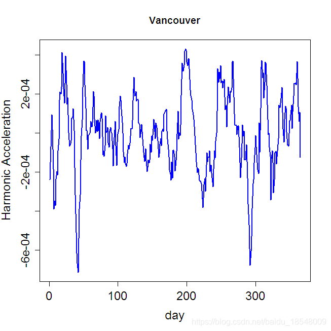
For Periodic data which is not very different from a sinusoid. The Harmonic acceleration of $x(t)$ is

$Lx(t) = \omega^2 D x(t) + D^3 x(t).$

Then $L cos(\omega t) = L sin(\omega t) = 0$.

We can measure departures form a sinusoid by

$J_L(x) = \int \big[ Lx(t) \big]^2 ~ dt.$

Harmonic acceleration in vancouver precipitation

2.4.3 A very general notion

We can be even more general and allow roughness penalties to use any linear differential operator:

$Lx(t) = \sum_{k = 1}^m \alpha_m (t) D^m x(t).$

Then $x$ is “smooth” if $Lx(t) = 0$.

We will see later on that we can even ask the data to tell us what should be smooth. However, we will rarely need to use anything so sophisticated.

2.4.4 Linear smooths and degrees of freedom

• In least squares fitting, the degrees of freedom used to smooth the data is exactly $k$, the number of basis functions.

• In penalized smoothing, we can have $k > n$.

• The smoothing penalty reduces the flexibility of the smooth (i.e. we know something).

• The degrees of freedom are controlled by $\lambda$. A natural measure turns to be

  $$\begin{aligned} df(\lambda) &= traceS_\lambda, \\ S_\lambda &= \mathbf{\Phi} \big[ \mathbf{\Phi}^T \mathbf{\Phi} + \lambda R \big]^{-1} \mathbf{\Phi}^T. \end{aligned}$$

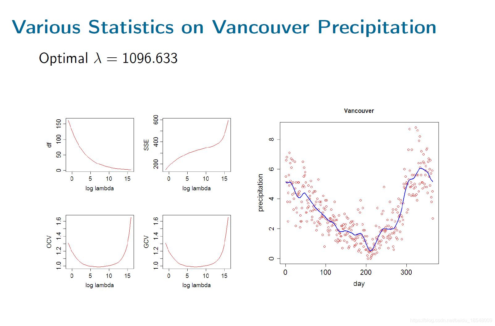
  Vancouver precipitation above was fit with 365 basis functions, and $\lambda = 10^4$ resulting in $df = 12.92$.

2.4.5 Choosing the smoothing parameters: Cross Validation

There are a number of data-driven methods for choosing smoothing parameters.

• Ordinary Cross Validation: leave one point out and see how well you can predict it. For any linear smooth

  $$\begin{aligned} OCV(\lambda) &= \sum \big(y_i - \hat{x}_{-i}(t_i) \big)^2 \\ &= \frac{1}{n} \sum \frac{\big( y_i - x_{\lambda} (t_i) \big)^2}{1 - S_{\lambda (ii)}}. \end{aligned}$$

  where $S$ is the smoothing matrix.

• Generalized cross validation:

  $$\begin{aligned} GCV(\lambda) &= \frac{n^{-1} \sum \big( y_i - x(t_i) \big)^2}{[n^{-1} trace(I - S)]^2} \\ &= \Big( \frac{n}{n - df(\lambda)} \Big) \Big( \frac{SSE}{n - df(\lambda)} \Big). \end{aligned}$$

  $SSE$ is discounted for degrees of freedom like usual, but we them also make a discount for minimizing over $\lambda$.

  $GCV$ smooths more than $OCV$; even then, it may need to be tweaked a little to produce pleasing results.

• Various information criteria: $AIC$, $BIC$…

• ReML estimation

2.5 Summary

Smoothing penalities used to penalize roughness of the result.

• $Lx(t) = 0$ defines what is smooth.

• Commonly $Lx(t) = D^2x(t) \Rightarrow$ straight lines are smooth.

• Alternative: $Lx(t) = D^3 x(t) + w^2 Dx(t) \Rightarrow$ sinusoids are smooth.

• Departures from smoothness traded off against fit to data.

• $GCV$ used to dicide on trade off; other possibilities availabe.

3 Descriptive statistics for functional data

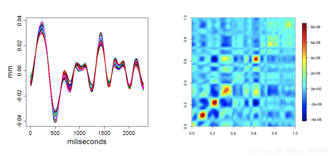
Summary statistics:

• Mean: $\bar{x} (t) = \frac{1}{n} \sum x_i(t);$

• Covariance: $\begin{aligned} \sigma (s, t) &= cov(x(s), x(t)) \\\\ &= \frac{1}{n} \sum \big( x_i (s) - \bar{x}(s) \big) \big( x_i (t) - \bar{x}(t) \big); \end{aligned}$ Covariance surfaces provide insight but do not describe the major directions of variation;

• Correlation:

$\rho(s, t) = \frac{\sigma (s, t)}{\sqrt{\sigma (s, s)} \sqrt{\sigma (t, t)}}.$

4 R example

4.1 New functions

Package “fda”.pdf

Functions used	Detials
smooth.basis()
int2Lfd()	Convert integer to linear differential operator
vec2Lfd(vectorCoef, rangeval = vectorRange)	Make a linear differential operator object from a vector
fdPar()	Define a functional parameter object
plotfit.fd
“
“
“
“
“
“

Firstly, load up the library and the data.

par(ask = FALSE)
library("fda")

data(CanadianWeather)

temp <- CanadianWeather$dailyAv[ , , 1]
precip <- CanadianWeather$dailyAv[ , , 2]

daytime <- (1:365) - 0.5
day5 <- seq(0, 365, 5)

dayrng <- c(0, 365)

Fit the temperature data with b-spline basis without smoothing.

bbasis <- create.bspline.basis(dayrng, nbasis = 21, norder = 4)

tempSmooth1 <- smooth.basis(daytime, temp, bbasis)

plot(tempSmooth1)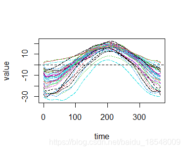

Using smooth functions.

4.1 Lfd objects

# Two common means of generating Lfd objects.

# 1/ int2Lfd -- just penalize some derivatives.
curv.Lfd <- int2Lfd(2)  # penalize the squared acceleration

# 2/ vec2Lfd -- a (constant) linear combination of derivatives; for technical
# reasons this also requires the range of the basis.
harm.Lfd <- vec2Lfd(c(0, (2*pi/365)^2, 0), rangeval = dayrng)

Looking inside these objects is not terribly enlightening.

4.2 fdPar objects

We’ll concentrate on B-splines and second-derivative penalties.

# First, a value of lambda  (purposefully large so that we can distinguish a 
# fit from data below).
lambda <- 1e6

# Now define the fdPar object.
curv.fdPar <- fdPar(bbasis, curv.Lfd, lambda)

4.3 Smoothing functions

# We're now in a position to smooth.
tempSmooth1 <- smooth.basis(daytime, temp, curv.fdPar)

# Let's look at the result.
names(tempSmooth1)
# [1] "fd"      "df"      "gcv"     "beta"    "SSE"     "penmat"  "y2cMap" 
# [8] "argvals" "y"   

# Plot it.
plot(tempSmooth1$fd)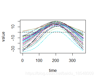

# There is also a neat utility to go through each curve in turn and look at 
# its fit to the data.
par(mfrow = c(2,2))
plotfit.fd(temp, daytime, tempSmooth1$fd, index = 1:4)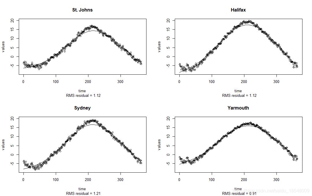

4.4 Examine some fit statistics

# degrees of freedom
tempSmooth1$df
# [1] 5.06577

# Just about equivalent to fitting 5 parameters.

# We'll also look at GCV, this is given for each observation.
tempSmooth1$gcv
# St. Johns      Halifax       Sydney     Yarmouth   Charlottvl  Fredericton 
# 1.2795697    1.2916752    1.5058050    0.8453872    1.5282543    1.5145976 
# Scheffervll     Arvida  Bagottville       Quebec   Sherbrooke     Montreal 
# 2.1866513    2.0339306    1.8815098    1.5730488    1.8063912    1.6288147 
#    Ottawa      Toronto       London  Thunder Bay     Winnipeg      The Pas 
# 1.6414521    1.4650397    1.4648668    1.4939418    1.9590623    2.0175589 
# Churchill       Regina   Pr. Albert Uranium City     Edmonton      Calgary 
# 2.5650108    1.7818144    2.1515356    3.4367165    1.9083830    1.5607955 
#  Kamloops    Vancouver     Victoria   Pr. George   Pr. Rupert   Whitehorse 
# 0.9614403    0.4837343    0.4492183    0.9754061    0.4195135    1.9692874 
#    Dawson  Yellowknife      Iqaluit       Inuvik     Resolute 
# 3.6711783    3.6956002    2.9828132    6.8113863    4.7486237 

4.5 A more realistic value of lambda

lambda <- 1e1
curv.fdPar$lambda <- lambda
tempSmooth <- smooth.basis(daytime, temp, curv.fdPar)

#Repeat the previous steps
par(mfrow = c(2,2))
plotfit.fd(temp, daytime, tempSmooth$fd, index = 1:4)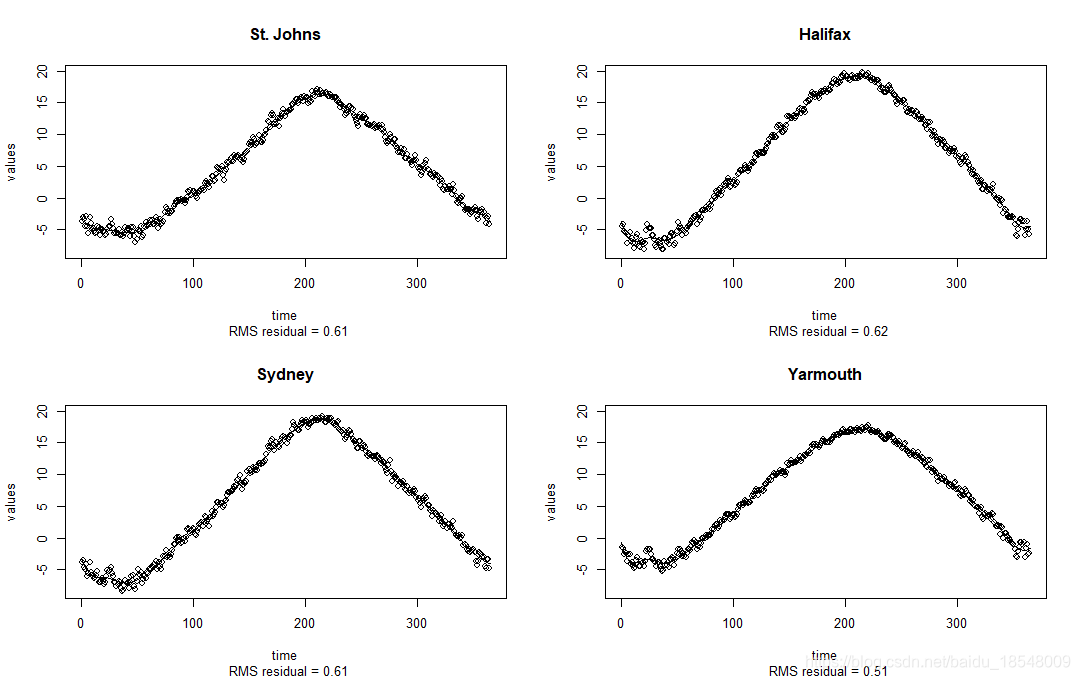

tempSmooth$df
# [1] 20.88924

tempSmooth$gcv
# St. Johns      Halifax       Sydney     Yarmouth   Charlottvl  Fredericton 
# 0.4186354    0.4301329    0.4209142    0.2948393    0.4788182    0.5038863 
# Scheffervll     Arvida  Bagottville       Quebec   Sherbrooke     Montreal 
# 0.6742076    0.8735580    0.6212167    0.4722118    0.7790845    0.5541590 
#    Ottawa      Toronto       London  Thunder Bay     Winnipeg      The Pas 
# 0.5271093    0.4824045    0.4844556    0.4354220    0.5641720    0.5892378 
# Churchill       Regina   Pr. Albert Uranium City     Edmonton      Calgary 
# 0.6442146    0.5819684    0.6429497    1.0420690    0.6471629    0.7837149 
#  Kamloops    Vancouver     Victoria   Pr. George   Pr. Rupert   Whitehorse 
# 0.3360671    0.1172343    0.1318441    0.5298761    0.1653976    1.0228183 
#    Dawson  Yellowknife      Iqaluit       Inuvik     Resolute 
# 1.0459365    0.7375391    0.5248940    1.0594254    0.3209614 

Here the fit looks a lot better and the gcv values are much smaller.

4.6 Choosing smoothing parameters

We can search through a collection of smoothing parameters to try and find an optimal parameter.

We will record the average gcv and choose lambda to be the minimum of these.

lambdas <- 10^seq(-4, 4, by = 0.5)  # lambdas to look over
mean.gcv <- rep(0, length(lambdas))  # store mean gcv

for(ilam in 1:length(lambdas)){
  # Set lambda
  curv.fdPari <- curv.fdPar
  curv.fdPari$lambda <- lambdas[ilam]

  # Smooth
  tempSmoothi <- smooth.basis(daytime, temp, curv.fdPari)
  
  # Record average gcv
  mean.gcv[ilam] <- mean(tempSmoothi$gcv)
}

# We can plot what we have
par(mfrow = c(1, 1))
plot(lambdas, mean.gcv, type = 'b', log = 'x')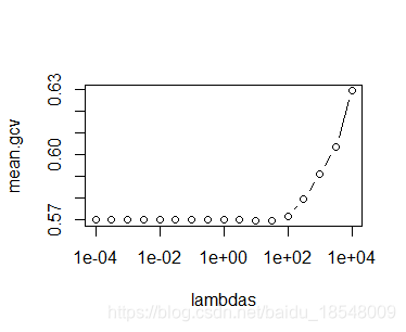

Select the lowest of these and smooth.

best <- which.min(mean.gcv)
lambdabest <- lambdas[best]
curv.fdPar$lambda <- lambdabest
tempSmooth <- smooth.basis(daytime, temp, curv.fdPar)

And look at the same statistics

par(mfrow = c(2,2))
plotfit.fd(temp, daytime, tempSmooth$fd, index = 1:4)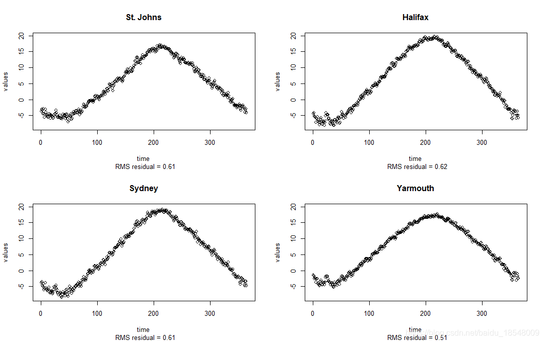

tempSmooth$df
# [1] 20.67444

# We'll also plot these
par(mfrow = c(1, 1))
plot(tempSmooth)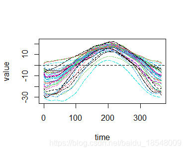

Functional data objects: manipulations and statistics

Now that we have a functional data object we can manipulate them in various ways. First let’s extract the fd object.